


Every developer loves a blazing-fast application. But what happens when that supposedly optimized, lightning-fast app crashes in production because it ate up all of the server’s available RAM? Memory management matters just as much as execution speed. To build truly scalable software, you must understand exactly how your algorithms consume physical resources under heavy loads. Welcome to the world of algorithm analysis.
What is Space Complexity?
Have you ever wondered exactly what space complexity is in the grand scheme of algorithm design? Simply put, it measures the total amount of memory an algorithm needs to run to completion, evaluated relative to the size of its input (typically denoted as n). But what is space complexity made of on a fundamental level? It is not just about the raw data you pass into a function. It consists of multiple moving parts that dictate how efficiently your code runs.
Breaking Down Memory Usage
To fully grasp this concept, we must split the memory footprint into two distinct categories.
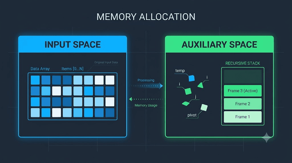
Input Space vs. Auxiliary Space
- Input Space: This is the memory allocated strictly to hold the initial input values. You cannot avoid this; if you process a list of one thousand integers, you must store one thousand integers.
- Auxiliary Space: This is the extra, temporary memory an algorithm uses during its execution. This includes temporary loop variables, newly allocated arrays, or frames on the recursive call stack.
When developers urgently ask what is space complexity during a code review, they are almost always concerned with this auxiliary overhead. Understanding what is space complexity at this granular level is the primary way software engineers prevent disastrous memory leaks in long-running applications.
Balancing Time and Space Complexity
There is a classic, unavoidable duality in computer science. Optimizing your code for speed almost always inflates its memory usage, and vice versa. Evaluating time and space complexity together is a mandatory skill for senior engineers.

Consider memoization. Caching previous calculation results radically speeds up execution because the CPU does not have to repeat the same work twice. However, storing those cached results demands significantly more memory. If you casually ignore the delicate balance of time and space complexity, your application might become fast but incredibly resource-hungry. Developers must consistently analyze time and space complexity simultaneously to find the “sweet spot” for their specific hardware constraints.
When we look closely at space and time complexity tradeoffs in embedded systems—where memory is fiercely limited—we often choose slower algorithms simply to save RAM. Conversely, on modern cloud servers, we usually sacrifice memory to gain speed. Ignoring this vital balance of time and space complexity inevitably leads to poorly optimized code that cannot scale with user demand. Ultimately, mastering time and space complexity empowers you to write adaptable, future-proof software.
Understanding Time Complexity and Space Complexity
People frequently ask, what is time complexity and space complexity? While they sound strikingly similar, they measure entirely different dimensions of algorithm performance.
The core difference between time complexity and space complexity lies in their units of measurement. Time complexity calculates the total number of operations an algorithm performs as the input grows. Conversely, space complexity calculates the number of memory blocks (like bytes, words, or structural nodes) consumed.
When studying time complexity and space complexity, you must remember that an algorithm could be O(1) in time but O(n) in space, although that specific combination is rare. Usually, if you are actively analyzing time complexity and space complexity, you are looking at trade-offs between processing cycles and RAM capacity. To truly master algorithms and ace technical interviews, you have to weigh both time complexity and space complexity in your daily coding decisions. Overlooking either side of time complexity and space complexity is a guaranteed recipe for system bottlenecks.
Space Complexity in Data Structure
Let’s look at the foundational building blocks of software. Analyzing space complexity in data structure choices reveals exactly how different storage mechanisms impact memory allocation across your application.
Static vs. Dynamic Memory
Your space complexity in data structure design heavily depends on whether you implement static or dynamic memory allocation.
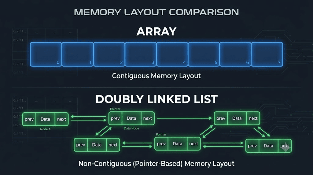
- Arrays: Arrays use static, contiguous memory. They are incredibly memory-efficient because they do not require extra metadata to store adjacent elements.
- Linked Lists: Linked lists rely on dynamic memory allocation. They require extra memory blocks for pointers (like next and prev references), which noticeably increases the overall space complexity in data structure implementations.
Evaluating Stacks and Trees
When traversing complex binary trees or utilizing stack structures, your space complexity in data structure choices dictate how deeply you can safely recurse before hitting a catastrophic stack overflow. Evaluating space complexity in data structure usage ensures your web servers won’t randomly crash when processing nested JSON objects or complex user data trees.
Analyzing Merge Sort Space Complexity
Sorting algorithms provide a fantastic, real-world lens for studying memory. Let’s closely examine divide-and-conquer strategies, specifically focusing on the space complexity of merge sort. Merge sort is famous in computer science for its highly reliable O(nn) time efficiency, but what about its physical memory footprint?
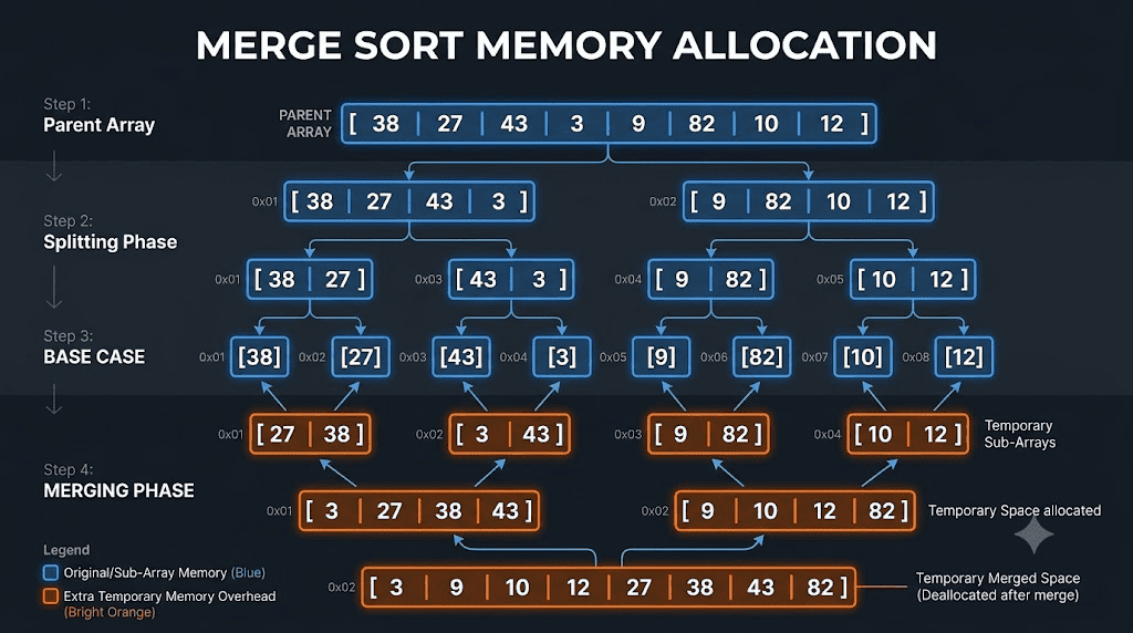
The space complexity of merge sort is exactly O(n) auxiliary space. Why does this happen? Because to merge the divided, smaller subarrays back together into a sorted whole, the algorithm must temporarily allocate new arrays that equal the size of the original input. This is exactly why reviewing the space complexity of merge sort is critical when handling massive datasets.
If you are sorting a messy database containing ten million user records, a merge sort space complexity of O(n) means you need enough available RAM to essentially duplicate that entire dataset during execution. Understanding the exact space complexity of merge sort helps you decide if your system can afford that heavy overhead, or if you need an in-place sorting algorithm like Heap Sort instead. Ultimately, the high space complexity of merge sort is its primary drawback compared to its peers.
Practical Application: Time and Space Complexity in Data Structure
Theory is great, but how does this apply to real-world engineering? The reality is that time and space complexity in data structure analysis guides every major architectural decision you make. Imagine you need to frequently search for active user IDs in a high-traffic web application.
When discussing time complexity and space complexity in data structure design, the hash map versus array debate is legendary. You essentially have two choices. Examining the time and space complexity in data structure tradeoffs provides the clear answer.
An unsorted array uses minimal extra memory (O(1) auxiliary space), but searching it takes O(n) time. If your list has a million users, that is a terribly slow search. A hash map, on the other hand, offers brilliant O(1) lookup time. However, it requires significantly more memory for underlying buckets and collision management.
This practical application of time and space complexity in data structure analysis clearly shows that you are always buying execution speed with physical memory. By deeply mastering time and space complexity in data structure principles, you can confidently defend your technical choices in complex system design interviews and daily team code reviews. Understanding these time and space complexity in data structure tradeoffs is ultimately what separates junior coders from seasoned, effective software architects.
FAQs
Q 1: What is the space complexity of binary search?
An iterative binary search requires O(1) constant auxiliary space because it only uses a few variables (like left, right, and mid pointers) to track the search boundaries. Conversely, a recursive implementation takes O(n) space due to the call stack frames. Every time the function calls itself, the system allocates new memory on the execution stack, making the space complexity of binary search heavily dependent on how you write the actual code.
Q 2: How do you calculate space complexity?
To understand how to calculate space complexity, you must sum up all auxiliary variables, object pointers, temporary arrays, and recursive stack frames utilized during execution. You evaluate this total memory requirement in terms of the input size n. Just like evaluating time efficiency with Big-O notation, you drop all constants and lower-order terms to find the dominant memory growth rate as the input scales toward infinity.
Q 3: What is the space complexity of quick sort?
The space complexity of quick sort is typically O(n) auxiliary space on average. This memory overhead comes directly from the recursive partitioning stack calls. Because it sorts in-place, it doesn’t need to duplicate arrays like merge sort. However, if you choose a poor pivot element on an already sorted array, the worst-case recursive depth can degrade to O(n) auxiliary space, which can easily trigger a stack overflow error.







Leave a Reply